Use Summary Functions to Summarize Data in Excel

For those who use Excel regularly, the number of built-in formulas and functions to summarize and manipulate data is staggering. Excel is literally used by everyone: from students in a financial class to hedge fund managers on Wall Street. It’s extremely powerful, but at the same time very simple.

For those just getting started with Excel, one of the first group of functions you should learn are the summary functions. These include SUM, AVERAGE, MAX, MIN, MODE, MEDIAN, COUNT, STDEV, LARGE, SMALL and AGGREGATE. These functions are best used on numerical data.

In this article, I’ll show you how to create a formula and insert the function into an Excel spreadsheet. Each function in Excel takes arguments, which are the values the functions needs to calculate an output.

Understanding Formulas & Functions

For example, if you need to add 2 and 2 together, the function would be SUM and the arguments would be the numbers 2 and 2. We normally write this as 2 + 2, but in Excel you would write it as =SUM(2+2). Here you can see the results of this simple addition of two literal numbers.

Even though there is nothing wrong with this formula, it really isn’t necessary. You could just type =2+2 in Excel and that would work also. In Excel, when you use a function like SUM, it makes more sense to use arguments. With the SUM function, Excel is expecting at least two arguments, which would be references to cells on the spreadsheet.

How do we reference a cell inside the Excel formula? Well, that’s pretty easy. Every row has a number and every column has a letter. A1 is the first cell on the spreadsheet at the top left. B1 would be the cell to the right of A1. A2 is the cell directly below A1. Easy enough right?

Before we write our new formula, let’s add some data in columns A and B to work with. Go ahead and type random numbers from A1 to A10 and B1 to B10 for our data set. Now go to D1 and type in =SUM(A1,B1). You should see the result is simply the value of A1 + B1.

There are a couple of things to note while typing a formula in Excel. Firstly, you’ll notice that when you type the first opening parenthesis ( after the function name, Excel will automatically tell you what arguments that function takes. In our example, it shows number1, number2, etc. You separate arguments with commas. This particular function can take an infinite number of values since that is how the SUM function works.

Secondly, either you can type in the cell reference manually (A1) or you can click on the cell A1 after you typed the open parenthesis. Excel will also highlight the cell in the same color as the cell reference so you can see the corresponding values exactly. So we summed one row together, but how can we sum all the other rows without typing the formula again or copying and pasting? Luckily, Excel makes this easy.

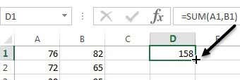
Move your mouse cursor to the bottom right corner of cell D1 and you’ll notice it changes from a white cross to a black plus sign.

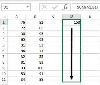
Now click and hold your mouse button down. Drag the cursor down to the last row with the data and then let go at the end.

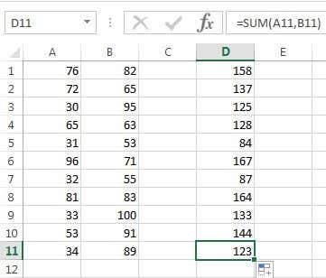
Excel is smart enough to know that the formula should change and reflect the values in the other rows rather than just showing you the same A1 + B1 all the way down. Instead, you’ll see A2+B2, A3+B3 and so on.

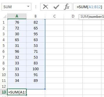
There is also another way to use SUM that explains another concept behind arguments in Excel. Let’s say we wanted to sum up all the values from A1 to A12, then how would we go about it? We could type something like =SUM(A1, A2, A3, etc), but that is very time consuming. A better way is to use an Excel range.

To sum A1 to A12, all we have to do is type =SUM(A1:A12) with a colon separating the two cell references instead of a comma. You could even type something like =SUM(A1:B12) and it will sum all values in A1 thru A12 and B1 thru B12.

This was a very basic overview of how to use functions and formulas in Excel, but it’s enough so that you can start using all of the data summation functions.

Summary Functions

Using the same set of data, we’re going to use the rest of the summary functions to see what kind of numbers we can calculate. Let’s start with the COUNT and COUNTA functions.

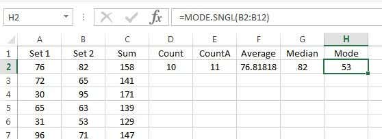
Here I have entered the COUNT function into D2 and the COUNTA function into E2, using A2:A12 range as the data set for both functions. I also changed the value in A9 to the text string hello to show the difference. COUNT only counts the cells that have numbers whereas COUNTA counts cells that contain text and numbers. Both functions do not count blank cells. If you want to count blank cells, use the COUNTBLANK function.

Next up are the AVERAGE, MEDIAN and MODE functions. Average is self-explanatory, median is the middle number in a set of numbers and mode is the most common number or numbers in a set of numbers. In newer versions of Excel, you have MODE.SNGL and MODE.MULT because there could be more than one number that is the most common number in a set of numbers. I used B2:B12 for the range in the example below.

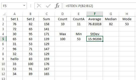
Moving on, we can calculate the MIN, MAX and STDEV for the set of numbers B2:B12. The STDEV function will calculate how widely values are dispersed from the average value. In newer versions of Excel, you have STDEV.P and STDEV.S, which calculates based on the entire population or based on a sample, respectively.

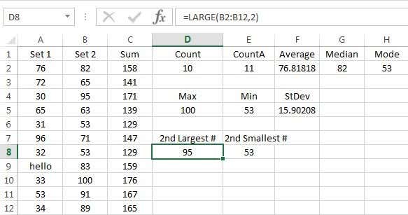
Finally, another two useful functions are LARGE and SMALL. They take two arguments: the cell range and the k-th largest value you want to return. So if you want the second largest value in the set, you would use 2 for the second argument, 3 for the third largest number, etc. SMALL works the same way, but gives you the k-th smallest number.

Lastly, there is a function called AGGREGATE, which allows you to apply any of the other functions mentioned above, but also lets you do things like ignore hidden rows, ignore error values, etc. You probably won’t need to use it that often, but you can learn more about it here in case you do need it.

So that’s a basic overview of some of the most common summary functions in Excel. If you have any questions, feel free to post a comment. Enjoy!