How to Insert and Use Bullet Points in Google Sheets

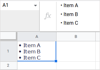
You might use bullet points in Microsoft Word or Google Docs to create a list. However, the options aren’t straightforward if you want to do the same in Google Sheets. So here, we’ll show you how to add bullet points in Google Sheets.

With four different methods for inserting bullet points, you can use whichever works best for your spreadsheet. These allow you to create lists within cells or add a bullet point in each separate cell to make an easy-to-read list.

Use a Keyboard Shortcut to Insert a Bullet

This method is ideal if you want to create a bullet list within a single cell. You’ll use keyboard shortcuts to insert the list. The keys you press depend on whether you use Windows or Mac.

Insert Bullets on Windows

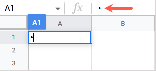
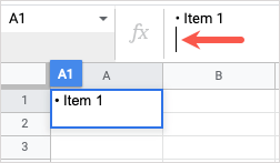
1. To add your first bullet point within a cell on Windows, select the cell and press Enter to display the cursor or go to the Formula Bar at the top.
2. Use the key combination Alt + 7 with the 7 being on your numeric keypad.

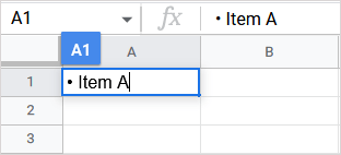
3. When you see the bullet point, you can insert your list item or add a space before the item if you like.

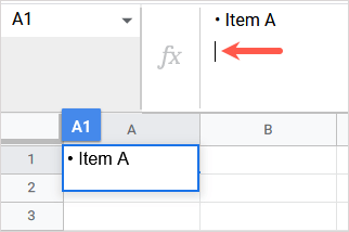
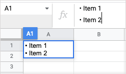
4. Use the key combination Alt + Enter to drop down to a new line within the cell.

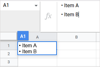
5. Then, follow Steps 2 and 3 above to enter another bullet point.

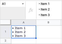
6. Continue this process until you complete the list. Then, press Enter.

Insert Bullets on Mac

1. To add your first bullet point within a cell on Mac, select the cell and use the key combination Option + 8.

2. When you see the bullet point, you can insert your list item or add a space before it.

3. Use the key combination Control + Return to add a line break within the cell.

4. Then, follow Steps 1 and 2 above to enter another bullet point.

5. Continue this process until you finish your list. Then, press Return.

Copy and Paste a Bullet

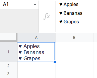
This next option also works if you want a bullet list in a cell but prefer something other than the default black dot, like an emoji or checkmark. You can also use this method to add bullets to individual cells if you like. You’ll simply copy and paste the symbol from another app.

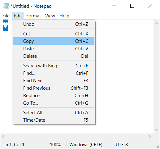
1. Select the symbol you want to use as a bullet from another spot on your computer. Then copy it using the menu or the keyboard shortcut Ctrl + C on Windows or Command + C on Mac.

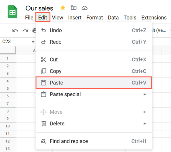
2. Choose the cell where you want to paste the symbol. Select Edit > Paste from the menu, right-click and pick Paste, or use a keyboard shortcut. Use Ctrl + V on Windows or Command + V on Mac.

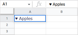
3. When the symbol appears in the cell, add your list item, with or without a space before it.

4. If you only want that one item in the cell, press Enter or Return and you’re set.
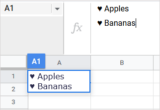
5. If you want to add another point within the cell, use Alt + Enter on Windows or Control + Return on Mac to add a new line.
6. Then, paste the symbol again and enter your next list item.

7. When you complete the list, press Enter or Return.

Enter the CHAR Function and Formula

Another way to insert bullets is by using the CHAR function and its formula in Google Sheets. The syntax for the formula is CHAR(number).

Use the Bullet List Number

If you simply want the default black dot for the bullet, the number is 9679. You then include the list item in the CHAR formula within quotes or using a cell reference. Let’s look at a couple of examples.

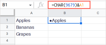
Here, we’ll use the text in cell A1 as our list item without a space using this formula:

=CHAR(9679)&A1

To break down the formula, you have CHAR(9679) for the bullet point, an ampersand to add to the string, and A1 for the text.

For another example, we’ll insert the bullet point and include a space with “abc” as our list item using this formula:

=CHAR(9679)&” “&”abc”

To break down this formula, you have CHAR(9679) for the bullet point, an ampersand to add to the string, a space enclosed in quotation marks, another ampersand, and the text within quotes.

Use a Unicode Character

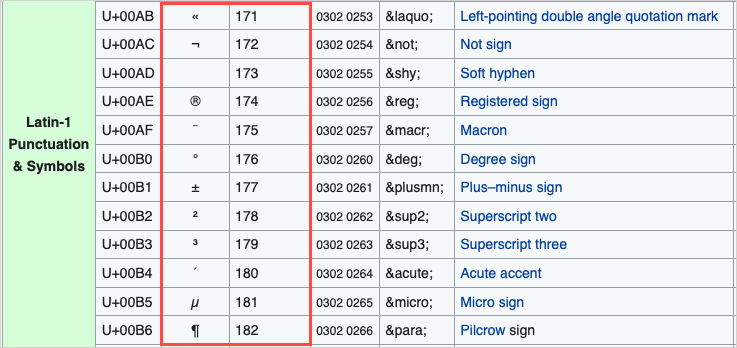
You can also use the Unicode number for the symbol you want in the formula. You can obtain the number from the List of Unicode Characters on Wikipedia or your own source.

As an example, we’ll use the Latin Letter Bilabial Click, which is number 664.

We’ll then add a space and “abc” as our list item with this formula:

=CHAR(664)&” “&”abc”

Create a Custom Number Format

This final method we’ll explain is perfect if you want to format existing cells with bullet points. You can create a custom number format that you then apply to any cells you like. Just note that it may affect the existing number formats you use for the cells.

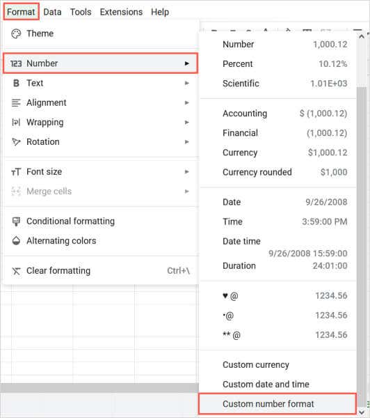
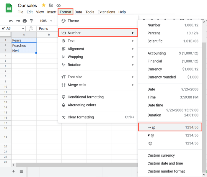
1. Select Format > Number and choose Custom number format at the bottom of the pop-out menu.

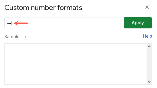
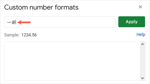
2. When the Custom Number Formats window opens, enter the symbol you want to use in the box at the top. You can use an asterisk, a dash, or paste a special symbol as described earlier.

3. If you want a space between the bullet and text, enter a space.
4. Then, add the @ (At) symbol.
5. Select Apply to save the format and apply it to the current cell.

6. When the window closes, you won’t see the symbol you included (if the cell is blank) until you type within the cell and press Enter or Return.

7. To apply the new format to other existing cells, select the cells, go to the Format menu, move to Number, and choose the format you created from the list.

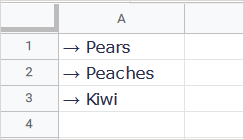
You’ll then see your selected cells update to use your custom bullet format.

You can also access and use the same custom format in other worksheets or Google Sheets workbooks when you sign in with the same Google account.

With these simple ways to insert bullet points in Google Sheets, you can easily create a list just like in Google Docs. For related tutorials, look at ways to use a checkmark in Microsoft Excel.