Some of these are similar to Excel
In early 2023, Google introduced several new functions for Sheets, including eight for working with arrays. Using these functions, you can transform an array into a row or column, create a new array from a row or column, or append a current array.
With more flexibility for working with arrays and going beyond the basic ARRAYFORMULA function, let’s look at how to use these array functions with formulas in Google Sheets.
Tip: Some of these functions may look familiar to you if you also use Microsoft Excel.
Transform an Array: TOROW and TOCOL
If you have an array in your dataset that you want to transform into a single row or column, you can use the TOROW and TOCOL functions.
The syntax for each function is the same, TOROW(array, ignore, scan) and TOCOL(array, ignore, scan) where only the first argument is required for both.
- Array: The array you want to transform, formatted as “A1:D4.”
- Ignore: By default, no parameters are ignored (0), but you can use 1 to ignore blanks, 2 to ignore errors, or 3 to ignore blanks and errors.
- Scan: This argument determines how to read the values in the array. By default, the function scans by row or using the value False, but you can use True to scan by column if you prefer.
Let’s walk through a few examples using the TOROW and TOCOL functions and their formulas.
In this first example, we’ll take our array A1 through C3 and turn it into a row using the default arguments with this formula:
=TOROW(A1:C3)
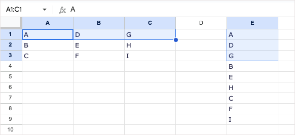
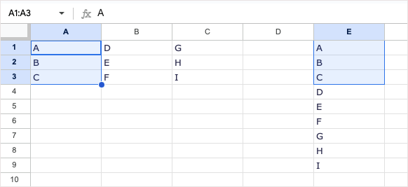
As you can see, the array is now in a row. Because we used the default scan argument, the function reads from left to right (A, D, G), down, then the left to right again (B, E, H) until complete—scanned by row.
To read the array by column instead of row, we can use True for the scan argument. We’ll leave the ignore argument blank. Here’s the formula:
=TOROW(A1:C3,,TRUE)
Now you see the function reads the array from top to bottom (A, B, C), top to bottom (D, E, F), and top to bottom (G, H, I).
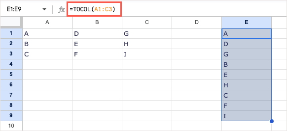
The TOCOL function works the same way but transforms the array to a column. Using the same range, A1 through C3, here’s the formula using the default arguments:
=TOCOL(A1:C3)
Again, using the default for the scan argument, the function reads from left to right and provides the result as such.
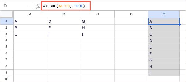
To read the array by column instead of row, insert True for the scan argument like this:
=TOCOL(A1:C3,,TRUE)
Now you see the function reads the array from top to bottom instead.
Related: Having trouble with formulas? Check out our guide to troubleshooting Google Sheets formula parse errors.
Create a New Array From Rows or Columns: CHOOSEROWS and CHOOSECOLS
You may want to create a new array from an existing one. This lets you make a new cell range with only specific values from another. For this, you’ll use the CHOOSEROWS and CHOOSECOLS Google Sheets functions.
The syntax for each function is similar, CHOOSEROWS (array, row_num, row_num_opt) and CHOOSECOLS (array, col_num, col_num_opt), where the first two arguments are required for both.
- Array: The existing array, formatted as “A1:D4.”
- Row_num or Col_num: The number of the first row or column you want to return.
- Row_num_opt or Col_num_opt: The numbers for additional rows or columns you want to return. Google suggests you use negative numbers to return rows from the bottom up or columns from right to left.
Let’s look at a few examples using CHOOSEROWS and CHOOSECOLS and their formulas.
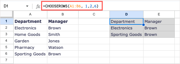
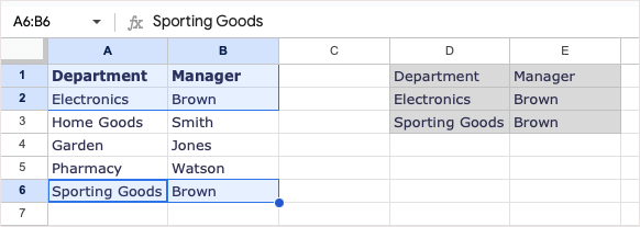
In this first example, we’ll use the array A1 through B6. We want to return the values in rows 1, 2, and 6. Here’s the formula:
=CHOOSEROWS(A1:B6,1,2,6)
As you can see, we received those three rows to create our new array.
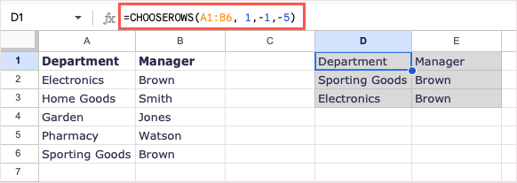
For another example, we’ll use the same array. This time, we want to return rows 1, 2, and 6 but with 2 and 6 in reverse order. You can use positive or negative numbers to receive the same result.
Using negative numbers, you’d use this formula:
=CHOOSEROWS(A1:B6,1,-1,-5)
To explain, 1 is the first row to return, -1 is the second row to return which is the first row starting at the bottom, and -5 is the fifth row from the bottom.
Using positive numbers, you’d use this formula to obtain the same result:
=CHOOSEROWS(A1:B6,1,6,2)
The CHOOSECOLS function works similarly, except you use it when you want to create a new array from columns instead of rows.
Using the array A1 through D6, we can return columns 1 (column A) and 4 (column D) with this formula:
=CHOOSECOLS(A1:D6,1,4)
Now we have our new array with only those two columns.
As another example, we’ll use the same array starting with column 4. We’ll then add columns 1 and 2 with 2 (column B) first. You can use either positive or negative numbers:
=CHOOSECOLS(A1:D6,4,2,1)
=CHOOSECOLS(A1:D6,4,-3,-4)
As you can see in the above screenshot, with the formulas in the cells rather than the Formula Bar, we receive the same result using both options.
Note: Because Google suggests using negative numbers to reverse the placement of the results, keep this in mind if you aren’t receiving the correct results using positive numbers.
Wrap to Create a New Array: WRAPROWS and WRAPCOLS
If you want to create a new array from an existing one but wrap the columns or rows with a certain number of values in each, you can use the WRAPROWS and WRAPCOLS functions.
The syntax for each function is the same, WRAPROWS (range, count, pad) and WRAPCOLS (range, count, pad), where the first two arguments are required for both.
- Range: The existing cell range you want to use for an array, formatted as “A1:D4.”
- Count: The number of cells for each row or column.
- Pad: You can use this argument to place text or a single value in empty cells. This replaces the #N/A error you’ll receive for the blank cells. Include the text or value within quotation marks.
Let’s walk through a few examples using the WRAPROWS and WRAPCOLS functions and their formulas.
In this first example, we’ll use the cell range A1 through E1. We’ll create a new array wrapping rows with three values in each row. Here’s the formula:
=WRAPROWS(A1:E1,3)
As you can see, we have a new array with the correct result, three values in each row. Because we have an empty cell in the array, the #N/A error displays. For the next example, we’ll use the pad argument to replace the error with the text “None.” Here’s the formula:
=WRAPROWS(A1:E1,3,”None”)
Now, we can see a word instead of a Google Sheets error.
The WRAPCOLS function does the same thing by creating a new array from an existing cell range, but does so by wrapping columns instead of rows.
Here, we’ll use the same array, A1 through E3, wrapping columns with three values in each column:
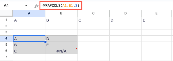
=WRAPCOLS(A1:E1,3)
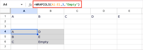
Like the WRAPROWS example, we receive the correct result but also an error because of the empty cell. With this formula, you can use the pad argument to add the word “Empty”:
=WRAPCOLS(A1:E1,3,”Empty”)
This new array looks much better with a word instead of the error.
Combine to Create a New Array: HSTACK and VSTACK
Two final functions we’ll look at are for appending arrays. With HSTACK and VSTACK, you can add two or more ranges of cells together to form a single array, either horizontally or vertically.
The syntax for each function is the same, HSTACK (range1, range2,…) and VSTACK (range1, range2,…), where only the first argument is required. However, you’ll almost always use the second argument, which combines another range with the first.
- Range1: The first cell range you want to use for the array, formatted as “A1:D4.”
- Range2,…: The second cell range you want to add to the first to create the array. You can combine more than two cell ranges.
Let’s look at some examples using HSTACK and VSTACK and their formulas.
In this first example, we’ll combine the ranges A1 through D2 with A3 through D4 using this formula:
=HSTACK(A1:D2,A3:D4)
You can see our data ranges combined to form a single horizontal array.
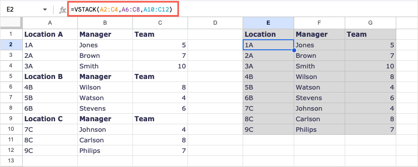
For an example of the VSTACK function, we combine three ranges. Using the following formula, we’ll use ranges A2 through C4, A6 through C8, and A10 through C12:
=VSTACK(A2:C4,A6:C8,A10:C12)
Now, we have one array with all of our data using a formula in a single cell.
Manipulate Arrays With Ease
While you can use ARRAYFORMULA in certain situations, like with the SUM function or IF function, these additional Google Sheets array formulas can save you time. They help you arrange your sheet exactly as you want it and with a single array formula.
For more tutorials like this, but with non-array functions, look at how to use the COUNTIF or SUMIF function in Google Sheets.

